Prepare Sports Injury Data

library(injurytools)
library(dplyr)

Data preprocessing is the very first step one has to follow, every time one wants to analyze sports injury data using injurytools R package.

This document briefly shows how to use the functions intended to facilitate this data preprocessing step and what the final data set is like.

Starting point

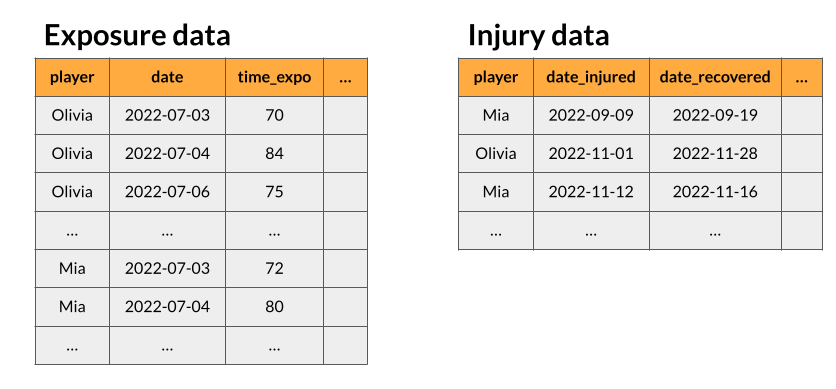
Data can be collected in several ways and by several means. A conventional manner is to collect and store data as events occur. So, with regard to sports medicine, it is common to store injury records on one hand, and on the other side, data related to training and competitions/matches (exposure time among others) in a separate table. Following this, we consider that the user has the raw data in two separate data sets that we call injury and exposure data, respectively¹.

1) prepare and standardize injury and exposure data

Thus the early task is to tidy up these two sources of data.

As example data sets we consider raw_df_injuries and raw_df_exposures data sets available from the injurytools package. These are data of Liverpool Football Club male’s first team players over two consecutive seasons, 2017-2018 and 2018-2019, scrapped from https://www.transfermarkt.com/ website:

head(raw_df_injuries)
#> # A tibble: 6 × 11
#>   player_name player_id season from       until      days_lost games_lost injury
#>   <fct>       <fct>     <fct>  <date>     <date>         <dbl>      <dbl> <chr> 
#> 1 adam-lalla… 43530     17/18  2017-07-31 2017-11-25       117         21 Hamst…
#> 2 adam-lalla… 43530     17/18  2018-03-31 2018-05-13        43         11 Hamst…
#> 3 adam-lalla… 43530     18/19  2018-09-04 2018-10-19        45          7 Groin…
#> 4 adam-lalla… 43530     18/19  2018-11-09 2018-12-04        25          4 Knock 
#> 5 adam-lalla… 43530     18/19  2019-01-06 2019-01-18        12          2 Knock 
#> 6 adam-lalla… 43530     18/19  2019-04-01 2019-05-31        60         10 Knock 
#> # ℹ 3 more variables: injury_acl <fct>, injury_type <fct>,
#> #   injury_severity <fct>
head(raw_df_exposures)
#>               player_name player_id season year matches_played minutes_played
#> 1            adam-lallana     43530  17/18 2017             12            236
#> 2            adam-lallana     43530  18/19 2018             13            464
#> 3          alberto-moreno    207917  17/18 2017             16           1264
#> 4 alex-oxlade-chamberlain    143424  17/18 2017             32           1483
#> 5                 alisson    105470  18/19 2018             38           3420
#> 6        andrew-robertson    234803  17/18 2017             22           1943
#>      liga    club_name club_id age height place citizenship
#> 1 premier fc-liverpool      31  29   1.72  <NA>        <NA>
#> 2 premier fc-liverpool      31  30   1.72  <NA>        <NA>
#> 3 premier fc-liverpool      31  25   1.71  <NA>        <NA>
#> 4 premier fc-liverpool      31  24   1.75  <NA>        <NA>
#> 5 premier fc-liverpool      31  26   1.91  <NA>        <NA>
#> 6 premier fc-liverpool      31  23   1.78  <NA>        <NA>
#>                     position  foot goals assists yellows reds
#> 1 Midfield_AttackingMidfield  both     0       0       1    0
#> 2 Midfield_AttackingMidfield  both     0       0       1    0
#> 3          Defender_LeftBack  left     0       0       1    0
#> 4   Midfield_CentralMidfield right     3       7       3    0
#> 5                 Goalkeeper right     0       0       1    0
#> 6          Defender_LeftBack  left     1       5       2    0

We standardize the key column names such as: player (subject) identifier, dates of injury and recovery (if any), training/match/season date and amount of time of exposure. And set them proper names and formats by means of prepare_inj() and prepare_exp()².

df_injuries <- prepare_inj(df_injuries0   = raw_df_injuries,
                           player         = "player_name",
                           date_injured   = "from",
                           date_recovered = "until")

df_exposures <- prepare_exp(df_exposures0 = raw_df_exposures,
                            player        = "player_name",
                            date          = "year",
                            time_expo     = "minutes_played")

We suggest collecting exposure time on as fine scale as possible, i.e. minutes would be the desired unit as the total time spent training and participating in competitions/matches. However, if the units are “seasons”, then do:

See the R-code

## a possible way for the case where each row in exposure data correspond to a
## season and there is no more information about time of exposure
raw_df_exposures$time_expo_aux <- 1 
df_exposures2 <- prepare_exp(df_exposures0 = raw_df_exposures,
                             player        = "player_name",
                             date          = "year",
                             time_expo     = "time_expo_aux")

## note 'tstart_s' and 'tstop_s' columns
injd <-  prepare_all(data_exposures = df_exposures2,
                     data_injuries  = df_injuries,
                     exp_unit = "seasons")
head(injd)
#> # A tibble: 6 × 19
#>   player t0         tf         date_injured date_recovered tstart     tstop     
#>   <fct>  <date>     <date>     <date>       <date>         <date>     <date>    
#> 1 adam-… 2017-07-01 2019-06-30 2017-07-31   2017-11-25     2017-07-01 2017-07-31
#> 2 adam-… 2017-07-01 2019-06-30 2018-03-31   2018-05-13     2017-11-25 2018-03-31
#> 3 adam-… 2017-07-01 2019-06-30 2018-09-04   2018-10-19     2018-05-13 2018-09-04
#> 4 adam-… 2017-07-01 2019-06-30 2018-11-09   2018-12-04     2018-10-19 2018-11-09
#> 5 adam-… 2017-07-01 2019-06-30 2019-01-06   2019-01-18     2018-12-04 2019-01-06
#> 6 adam-… 2017-07-01 2019-06-30 2019-04-01   2019-05-31     2019-01-18 2019-04-01
#> # ℹ 12 more variables: tstart_s <dbl>, tstop_s <dbl>, status <dbl>, enum <dbl>,
#> #   days_lost <dbl>, player_id <fct>, season <fct>, games_lost <dbl>,
#> #   injury <chr>, injury_acl <fct>, injury_type <fct>, injury_severity <fct>

2) integrate both sources of data

Then, we apply prepare_all() to the data sets tidied up above. It is important to specify the unit of exposure, i.e. the exp_unit argument, which must be one of “minutes”, “hours”, “days”, “matches_num”, “matches_minutes”, “activity_days” or “seasons”.

injd <-  prepare_all(data_exposures = df_exposures,
                    data_injuries  = df_injuries,
                    exp_unit = "matches_minutes")
head(injd)
#> # A tibble: 6 × 19
#>   player t0         tf         date_injured date_recovered tstart     tstop     
#>   <fct>  <date>     <date>     <date>       <date>         <date>     <date>    
#> 1 adam-… 2017-07-01 2019-06-30 2017-07-31   2017-11-25     2017-07-01 2017-07-31
#> 2 adam-… 2017-07-01 2019-06-30 2018-03-31   2018-05-13     2017-11-25 2018-03-31
#> 3 adam-… 2017-07-01 2019-06-30 2018-09-04   2018-10-19     2018-05-13 2018-09-04
#> 4 adam-… 2017-07-01 2019-06-30 2018-11-09   2018-12-04     2018-10-19 2018-11-09
#> 5 adam-… 2017-07-01 2019-06-30 2019-01-06   2019-01-18     2018-12-04 2019-01-06
#> 6 adam-… 2017-07-01 2019-06-30 2019-04-01   2019-05-31     2019-01-18 2019-04-01
#> # ℹ 12 more variables: tstart_minPlay <dbl>, tstop_minPlay <dbl>, status <dbl>,
#> #   enum <dbl>, days_lost <dbl>, player_id <fct>, season <fct>,
#> #   games_lost <dbl>, injury <chr>, injury_acl <fct>, injury_type <fct>,
#> #   injury_severity <fct>
# injd |> 
#   group_by(player) |> 
#   slice(1, n())

The outcome is a prepared data set, structured in a suitable way that is ready for its use by statistical modelling approaches. These data set will always have the columns listed below (standardized columns or created by the function), as well as further (optional) sports-related variables.

player: player identifier.
t0 and tf: the follow-up period of the corresponding player, i.e. player’s first and last dates observed (same value for each player).
date_injured and date_recovered: dates of injury and recovery of the corresponding observation (if any). Otherwise NA.
tstart and tstop: beginning and ending dates of the corresponding interval in which the observation has been at risk of injury.
tstart_xand tstop_x: beginning and ending times of the corresponding interval in which the observation has been at risk of injury (it depends on the unit of exposure time specified).
status: injury (event) indicator.
enum: an integer indicating the recurrence number, i.e. the \(k\)-th injury (event), at which the observation is at risk.
days_lost: number of days lost due to injury occurred at tstop/date_injured (if any; otherwise 0), i.e. date_recovered - date_injured in days.

For example the first row of injd corresponds to the player Adam Lallana, to the risk set that starts on 2017-07-01 and ends on 2017-07-31, after having played 236 minutes, when he got firstly (enum = 1) injured (status = 1). The second row corresponds to the risk set of being injured by a second injury (enum = 2), the set starts when he was fully recovered in 2017-11-23 and finishes when he suffered another hamstring injury³.

The prepared data set, an `injd` object

These final data set it’s an R object of class injd,

class(injd)
#> [1] "injd"       "tbl_df"     "tbl"        "data.frame"

and have the following attributes:

str(injd, 1)
#> injd [108 × 19] (S3: injd/tbl_df/tbl/data.frame)
#>  - attr(*, "unit_exposure")= chr "matches_minutes"
#>  - attr(*, "follow_up")= tibble [28 × 3] (S3: tbl_df/tbl/data.frame)
#>  - attr(*, "data_exposures")='data.frame':   42 obs. of  19 variables:
#>  - attr(*, "data_injuries")= tibble [82 × 11] (S3: tbl_df/tbl/data.frame)

unit_exposure: a character indicating the unit of exposure time used in this object.
follow_up: a data frame consisting of one row per player with their first and last dates observed (t0 and tf columns).
data_exposures: the preprocessed exposure data frame.
data_injuries: the preprocessed injury data frame.

To extract one of the attributes, for example unit_exposure, type:

attr(injd, "unit_exposure")
#> [1] "matches_minutes"

2024-03-05

Starting point

1) prepare and standardize injury and exposure data

2) integrate both sources of data

The prepared data set, an injd object

The prepared data set, an `injd` object